


Introduction
The A* (A-star) algorithm is primarily used for pathfinding and graph traversal. It’s well-known for its effectivity in figuring out the shortest path. Fields resembling synthetic intelligence, robotics, and recreation growth depend on this algorithm.
The A* algorithm’s key power lies in its systematic exploration of a graph or grid. Ranging from an preliminary node, it effectively searches for the optimum path to the purpose node. This effectivity is achieved by combining the excellent nature of Dijkstra’s algorithm and the heuristic method of the Grasping Greatest-First Search.
The A* algorithm’s distinctive value perform units it aside. By contemplating each the precise value of reaching a node and an estimated heuristic of the remaining value, it intelligently prioritizes essentially the most promising paths. This twin consideration expedites the search, making it extremely correct and worthwhile.
Within the subsequent article, we’ll delve into detailed examples of the A* algorithm in motion, showcasing its effectiveness and flexibility.
By sustaining a proper tone and utilizing brief, concise sentences, this model conveys the important thing factors concerning the A* algorithm whereas retaining knowledgeable and technical focus.
Overview
- Describe the first use of A* in pathfinding and graph traversal.
- Clarify the fee perform parts: g(n)g(n)g(n), h(n)h(n)h(n), and f(n)f(n)f(n).
- Determine and differentiate between Manhattan, Euclidean, and Diagonal heuristics.
- Implement the A* algorithm in Python for grid-based pathfinding.
- Acknowledge A*’s purposes in AI, robotics, and recreation growth.
How Does the A* Algorithm Work?
The A* algorithm makes use of a mix of precise and heuristic distances to find out one of the best path. Listed here are the principle parts:
- g(n): The price of the trail from the beginning node to the present node nnn.
- h(n): A heuristic perform that estimates the fee from node nnn to the purpose.
- f(n): The overall estimated value of the trail by way of node nnn (f(n)=g(n)+h(n)f(n) = g(n) + h(n)f(n)=g(n)+h(n)).
A* Algorithm: Step-by-Step Information
Initialization
- Create an open listing to trace nodes for analysis.
- Make a closed listing for nodes which were evaluated.
- Add the beginning node to the open listing, marking the start of your path.
Most important Loop
- Proceed till the open listing is empty or the purpose is reached:
- Choose the node with the bottom f(x) worth, indicating essentially the most promising path.
- Transfer the chosen node from the open listing to the closed listing.
- Look at every neighbor of the chosen node to find out the following steps.
Evaluating Neighbors
- For every neighbor:
- If it’s the purpose, reconstruct the trail and return it as the answer.
- Skip any neighbors already within the closed listing, as they’ve been evaluated.
- If a neighbor isn’t within the open listing:
- Add it and calculate its g(x), h(x), and f(x) values.
- For neighbors already within the open listing:
- Verify if the brand new path is extra environment friendly (decrease g(x) worth).
- If that’s the case, replace the g(x), h(x), and f(x) values, and set the present node as its mother or father
Heuristics in A*
Heuristics are used to estimate the space from the present node to the purpose. Frequent heuristics embody:
- Manhattan Distance: Used when actions are restricted to horizontal and vertical instructions.
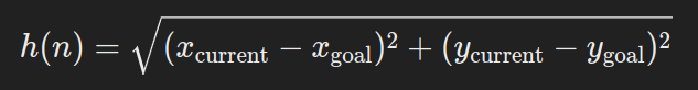
- Euclidean Distance: Used when actions might be in any course.
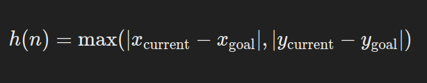
- Diagonal Distance: Used when actions might be in eight potential instructions (like a king in chess).
Implementing A* Algorithm in Python
Now, let’s see methods to implement the A* algorithm in Python. We’ll outline a easy grid-based map the place 0 represents walkable cells and 1 represents obstacles.
Code:
import heapq

import math

class Node:

    def __init__(self, place, mother or father=None):

        self.place = place

        self.mother or father = mother or father

        self.g = 0  # Distance from begin node

        self.h = 0  # Heuristic to purpose

        self.f = 0  # Whole value

    def __eq__(self, different):

        return self.place == different.place

    def __lt__(self, different):

        return self.f < different.f

    def __repr__(self):

        return f"({self.place}, f: {self.f})"

def heuristic(a, b):

    return math.sqrt((a[0] - b[0])**2 + (a[1] - b[1])**2)

def astar(maze, begin, finish):

    open_list = []

    closed_list = set()

    start_node = Node(begin)

    end_node = Node(finish)

    heapq.heappush(open_list, start_node)

    whereas open_list:

        current_node = heapq.heappop(open_list)

        closed_list.add(current_node.place)

        if current_node == end_node:

            path = []

            whereas current_node:

                path.append(current_node.place)

                current_node = current_node.mother or father

            return path[::-1]

        for new_position in [(0, -1), (0, 1), (-1, 0), (1, 0), (-1, -1), (-1, 1), (1, -1), (1, 1)]:

            node_position = (current_node.place[0] + new_position[0], current_node.place[1] + new_position[1])

            if node_position[0] > (len(maze) - 1) or node_position[0] < 0 or node_position[1] > (len(maze[len(maze)-1]) - 1) or node_position[1] < 0:

                proceed

            if maze[node_position[0]][node_position[1]] != 0:

                proceed

            new_node = Node(node_position, current_node)

            if new_node.place in closed_list:

                proceed

            new_node.g = current_node.g + 1

            new_node.h = heuristic(new_node.place, end_node.place)

            new_node.f = new_node.g + new_node.h

            if add_to_open(open_list, new_node):

                heapq.heappush(open_list, new_node)

    return None

def add_to_open(open_list, neighbor):

    for node in open_list:

        if neighbor == node and neighbor.g > node.g:

            return False

    return True

maze = [

    [0, 1, 0, 0, 0, 0, 0],

    [0, 1, 0, 1, 1, 1, 0],

    [0, 0, 0, 0, 0, 0, 0],

    [0, 1, 1, 1, 1, 1, 0],

    [0, 0, 0, 0, 0, 0, 0]

]

begin = (0, 0)

finish = (4, 6)

path = astar(maze, begin, finish)

print(path)
Output:
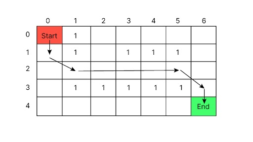
[(0, 0), (1, 0), (2, 1), (2, 2), (2, 3), (2, 4), (2, 5), (3, 6), (4, 6)]
Clarification of the Output
This path represents the sequence of steps from the place to begin (0, 0) to the endpoint (4, 6). Here’s a detailed step-by-step rationalization of the traversal:
- Begin at (0, 0): That is the preliminary place within the top-left nook of the maze.
- Transfer to (1, 0): Transfer one step right down to the primary row.
- Transfer to (2, 1): Transfer one step down and one step proper, avoiding the impediment in (1, 1).
- Transfer to (2, 2): Transfer one step proper.
- Transfer to (2, 3): Transfer one step proper.
- Transfer to (2, 4): Transfer one step proper.
- Transfer to (2, 5): Transfer one step proper.
- Transfer to (3, 6): Transfer diagonally down-right, skipping the obstacles and reaching the second final column within the third row.
Transfer to (4, 6): Transfer one step down to succeed in the purpose place.
Conclusion
This information has offered a complete overview of the A* algorithm’s performance together with code implementation. A* algorithm is a worthwhile instrument that simplifies complicated issues, providing a strategic and environment friendly method to discovering optimum options. I hope you discover this text useful in understanding this algorithm of python.
Incessantly Requested Questions
A. A* is an knowledgeable search algorithm, a sort of best-first search. It operates on weighted graphs, ranging from a particular node and aiming to seek out the optimum path to the purpose node. The algorithm considers varied elements, resembling distance and time, to determine the trail with the smallest total value.
A. The AO* algorithm employs AND-OR graphs to interrupt down complicated issues. The “AND” aspect of the graph represents interconnected duties important to reaching a purpose, whereas the “OR” aspect stands for particular person duties. This method simplifies problem-solving by figuring out process dependencies and standalone actions.
A. A* finds the shortest path in single-path issues utilizing a heuristic for value estimation. AO* handles AND-OR resolution graphs, fixing subproblems with mixed prices, excellent for complicated decision-making and game-playing eventualities.


/cdn.vox-cdn.com/uploads/chorus_asset/file/25588208/Megalopolis_Adam_Driver.png)


