Introduction
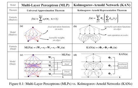
Kolmogorov-Arnold Networks, often known as KAN, are the most recent development in neural networks. Based mostly on the Kolgomorov-Arnold illustration theorem, they’ve the potential to be a viable different to Multilayer Perceptrons (MLP). Not like MLPs with fastened activation features at every node, KANs use learnable activation features on edges, changing linear weights with univariate features as parameterized splines.
A analysis group from the Massachusetts Institute of Expertise, California Institute of Expertise, Northeastern College, and The NSF Institute for Synthetic Intelligence and Elementary Interactions introduced Kolmogorov-Arnold Networks (KANs) as a promising substitute for MLPs in a latest paper titled “KAN: Kolmogorov-Arnold Networks.”
Studying Aims
- Be taught and perceive a brand new sort of neural community known as Kolmogorov-Arnold Community that may present accuracy and interpretability.
- Implement Kolmogorov-Arnold Networks utilizing Python libraries.
- Perceive the variations between Multi-Layer Perceptrons and Kolmogorov-Arnold Networks.
This text was printed as part of the Information Science Blogathon.
Kolmogorov-Arnold illustration theorem
In response to the Kolmogorov-Arnold illustration theorem, any multivariate steady perform might be outlined as:
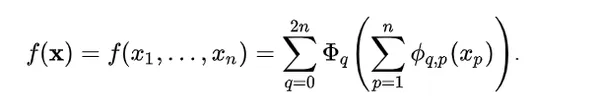
Right here:
ϕqp : [0, 1] → R and Φq : R → R
Any multivariate perform might be expressed as a sum of univariate features and additions. This would possibly make you suppose machine studying can grow to be simpler by studying high-dimensional features by way of easy one-dimensional ones. Nonetheless, since univariate features might be non-smooth, this theorem was thought-about theoretical and inconceivable in observe. Nonetheless, the researchers of KAN realized the potential of this theorem by increasing the perform to better than 2n+1 layers and for real-world, {smooth} features.
What are Multi-layer Perceptrons?
These are the only types of ANNs, the place data flows in a single course, from enter to output. The community structure doesn’t have cycles or loops. Multilayer perceptrons (MLP) are a kind of feedforward neural community.
Multilayer Perceptrons are a kind of feedforward neural community. Feedforward Neural Networks are easy synthetic neural networks during which data strikes ahead, in a single course, from enter to output by way of a hidden layer.
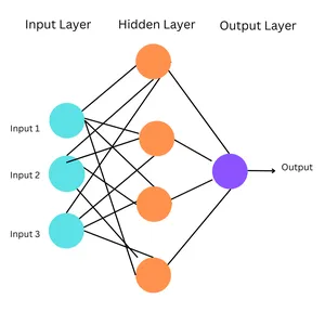
Working of MLPs
- Enter Layer: The enter layer consists of nodes representing the enter information’s options. Every node corresponds to 1 function.
- Hidden Layers: MLPs have a number of hidden layers between the enter and output layers. The hidden layers allow the community to study complicated patterns and relationships within the information.
- Output Layer: The output layer produces the ultimate predictions or classifications.
- Connections and Weights: Every connection between neurons in adjoining layers is related to a weight, figuring out its power. Throughout coaching, these weights are adjusted by way of backpropagation, the place the community learns to reduce the distinction between its predictions and the precise goal values.
- Activation Features: Every neuron (besides these within the enter layer) applies an activation perform to the weighted sum of its inputs. This introduces non-linearity into the community.
Simplified Formulation

Right here:
- σ = activation perform
- W = tunable weights that symbolize connection strengths
- x = enter
- B = bias
MLPs are based mostly on the common approximation theorem, which states {that a} feedforward neural community with a single hidden layer with a finite variety of neurons can approximate any steady perform on a compact subset so long as the perform is just not a polynomial. This permits neural networks, particularly these with hidden layers, to symbolize a variety of complicated features. Thus, MLPs are designed based mostly on this (with a number of hidden layers) to seize the intricate patterns in information. MLPs have fastened activation features on every node.
Nonetheless, MLPs have just a few drawbacks. MLPs in transformers make the most of the mannequin’s parameters, even these that aren’t associated to the embedding layers. They’re additionally much less interpretable. That is how KANs come into the image.
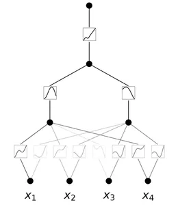
Kolmogorov-Arnold Networks (KANs)
A Kolmogorov-Arnold Community is a neural community with learnable activation features. At every node, the community learns the activation perform. Not like MLPs with fastened node activation features, KANs have learnable activation features on edges. They substitute the linear weights with parametrized splines.
Benefits of KANs
Listed here are the benefits of KANs:
- Better Flexibility: KANs are extremely versatile as a result of their activation features and mannequin structure, thus permitting higher illustration of complicated information.
- Adaptable Activation Features: Not like in MLPs, the activation features in KANs aren’t fastened. Since their activation features are learnable on edges, they will adapt and modify to totally different information patterns, thus successfully capturing various relationships.
- Higher Complexity Dealing with: They substitute the linear weights in MLPs by parametrized splines, thus they will deal with complicated, non-linear information.
- Superior Accuracy: KANs have demonstrated higher accuracy in dealing with high-dimensional information
- Extremely Interpretable: They reveal the buildings and topological relationships between the information thus they will simply be interpreted.
- Numerous Functions: they will carry out numerous duties like regression, partial differential equations fixing, and continuous studying.
Additionally learn: Multi-Layer Perceptrons: Notations and Trainable Parameters
Easy Implementation of KANs
Let’s implement KANs with the assistance of a easy instance. We’re going to create a customized dataset of the perform: f(x, y) = exp(cos(pi*x) + y^2). This perform takes two inputs, calculates the cosine of pi*x, provides the sq. of y to it, after which calculates the exponential of the end result.
Necessities of Python library model:
- Python==3.9.7
- matplotlib==3.6.2
- numpy==1.24.4
- scikit_learn==1.1.3
- torch==2.2.2
!pip set up git+https://github.com/KindXiaoming/pykan.git

import torch
import numpy as np

##create a dataset
def create_dataset(f, n_var=2, n_samples=1000, split_ratio=0.8):

    # Generate random enter information
    X = torch.rand(n_samples, n_var)

    # Compute the goal values
    y = f(X)

    # Cut up into coaching and take a look at units
    split_idx = int(n_samples * split_ratio)
    train_input, test_input = X[:split_idx], X[split_idx:]
    train_label, test_label = y[:split_idx], y[split_idx:]

    return {
        'train_input': train_input,
        'train_label': train_label,
        'test_input': test_input,
        'test_label': test_label
    }

# Outline the brand new perform f(x, y) = exp(cos(pi*x) + y^2)
f = lambda x: torch.exp(torch.cos(torch.pi*x[:, [0]]) + x[:, [1]]**2)

dataset = create_dataset(f, n_var=2)

print(dataset['train_input'].form, dataset['train_label'].form)
##output: torch.Measurement([800, 2]) torch.Measurement([800, 1])


from kan import *
# create a KAN: 2D inputs, 1D output, and 5 hidden neurons.
# cubic spline (okay=3), 5 grid intervals (grid=5).
mannequin = KAN(width=[2,5,1], grid=5, okay=3, seed=0)

# plot KAN at initialization
mannequin(dataset['train_input']);
mannequin.plot(beta=100)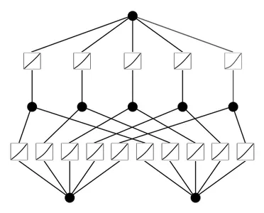
## prepare the mannequin

mannequin.prepare(dataset, choose="LBFGS", steps=20, lamb=0.01, lamb_entropy=10.)
## output: prepare loss: 7.23e-02 | take a look at loss: 8.59e-02
## output: | reg: 3.16e+01 : 100%|██| 20/20 [00:11<00:00,  1.69it/s]

mannequin.plot()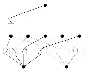
mannequin.prune()
mannequin.plot(masks=True)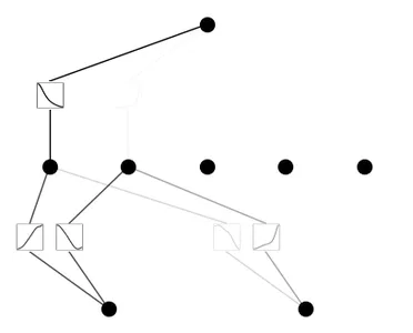
mannequin = mannequin.prune()
mannequin(dataset['train_input'])
mannequin.plot()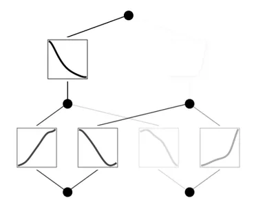
mannequin.prepare(dataset, choose="LBFGS", steps=100)
mannequin.plot()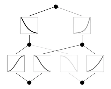
Code Clarification
- Set up the Pykan library from Git Hub.
- Import libraries.
- The create_dataset perform generates random enter information (X) and computes the goal values (y) utilizing the perform f. The dataset is then break up into coaching and take a look at units based mostly on the break up ratio. The parameters of this perform are:
- f: perform to generate the goal values.
- n_var: variety of enter variables.
- n_samples: complete variety of samples
- split_ratio: ratio to separate the dataset into coaching and take a look at units, and it returns a dictionary containing coaching and take a look at inputs and labels.
- Create a perform of the shape: f(x, y) = exp(cos(pi*x) + y^2)
- Name the perform create_dataset to create a dataset utilizing the beforehand outlined perform f with 2 enter variables.
- Print the form of coaching inputs and their labels.
- Initialize a KAN mannequin with 2-dimensional inputs, 1-dimensional output, 5 hidden neurons, cubic spline (okay=3), and 5 grid intervals (grid=5)
- Plot the KAN mannequin at initialization.
- Prepare the KAN mannequin utilizing the supplied dataset for 20 steps utilizing the LBFGS optimizer.
- After coaching, plot the skilled mannequin.
- Prune the mannequin and plot the pruned mannequin with the masked neurons.
- Prune the mannequin once more, consider it on the coaching enter, and plot the pruned mannequin.
- Re-train the pruned mannequin for an extra 100 steps.
MLP vs KAN
| MLP | KAN |
| Fastened node activation features | Learnable activation features |
| Linear weights | Parametrized splines |
| Much less interpretable | Extra interpretable |
| Much less versatile and adaptable as in comparison with KANs | Extremely versatile and adaptable |
| Sooner coaching time | Slower coaching time |
| Based mostly on Common Approximation Theorem | Based mostly on Kolmogorov-Arnold Illustration Theorem |
Conclusion
The invention of KANs signifies a step in the direction of advancing deep studying strategies. By offering higher interpretability and accuracy than MLPs, they could be a better option when interpretability and accuracy of the outcomes are the primary goal. Nonetheless, MLPs generally is a extra sensible resolution for duties the place pace is important. Analysis is constantly taking place to enhance these networks, but for now, KANs symbolize an thrilling different to MLPs.
The media proven on this article will not be owned by Analytics Vidhya and is used on the Writer’s discretion.
Continuously Requested Questions
A. Ziming Liu, Yixuan Wang, Sachin Vaidya, Fabian Ruehle, James Halverson, Marin Soljaci, Thomas Y. Hou, Max Tegmark are the researchers concerned within the dQevelopment of KANs.
A. Fastened activation features are mathematical features utilized to the outputs of neurons in neural networks. These features stay fixed all through coaching and will not be up to date or adjusted based mostly on the community’s studying. Ex: Sigmoid, tanh, ReLU.
Learnable activation features are adaptive and modified throughout the coaching course of. As an alternative of being predefined, they’re up to date by way of backpropagation, permitting the community to study probably the most appropriate activation features.
A. One limitation of KANs is their slower coaching time as a result of their complicated structure. They require extra computations throughout the coaching course of since they substitute the linear weights with spline-based features that require further computations to study and optimize.
A. In case your activity requires extra accuracy and interpretability and coaching time isn’t restricted, you may proceed with KANs. If coaching time is vital, MLPs are a sensible possibility.
A. The LBFGS optimizer stands for “Restricted-memory Broyden–Fletcher–Goldfarb–Shanno” optimizer. It’s a well-liked algorithm for parameter estimation in machine studying and numerical optimization.


/cdn.vox-cdn.com/uploads/chorus_asset/file/25547597/Screen_Shot_2024_07_26_at_3.55.30_PM.png)