Introduction
Exploratory Knowledge Evaluation (EDA) is a means of describing the info by way of statistical and visualization methods in an effort to deliver essential facets of that information into focus for additional evaluation. This entails inspecting the dataset from many angles, describing & summarizing it with out making any assumptions about its contents.
“Exploratory Knowledge evaluation is an perspective, a state of flexibility, a willingness to search for these issues that we imagine will not be there, in addition to these we imagine to be there”
– John W. Tukey
EDA is a major step to take earlier than diving into statistical modeling or machine studying, to make sure the info is basically what it’s claimed to be and that there are not any apparent errors. It ought to be a part of information science initiatives in each group.
Studying Goals
- Study what Exploratory Knowledge Evaluation (EDA) is and why it’s essential in information analytics.
- Perceive how to take a look at and clear information, together with coping with single variables.
- Summarize information utilizing easy statistics and visible instruments like bar plots to seek out patterns.
- Ask and reply questions concerning the information to uncover deeper insights.
- Use Python libraries like pandas, NumPy, Matplotlib, and Seaborn to discover and visualize information.
This text was revealed as part of the Knowledge Science Blogathon.
What’s Exploratory Knowledge Evaluation?
Exploratory Knowledge Evaluation (EDA) is like exploring a brand new place. You go searching, observe issues, and attempt to perceive what’s happening. Equally, in EDA, you have a look at a dataset, try the totally different elements, and take a look at to determine what’s taking place within the information. It entails utilizing statistics and visible instruments to know and summarize information, serving to information scientists and information analysts examine the dataset from varied angles with out making assumptions about its contents.
Right here’s a typical course of:
- Take a look at the Knowledge: Collect details about the info, such because the variety of rows and columns, and the kind of data every column incorporates. This consists of understanding single variables and their distributions.
- Clear the Knowledge: Repair points like lacking or incorrect values. Preprocessing is crucial to make sure the info is prepared for evaluation and predictive modeling.
- Make Summaries: Summarize the info to get a normal concept of its contents, resembling common values, widespread values, or worth distributions. Calculating quantiles and checking for skewness can present insights into the info’s distribution.
- Visualize the Knowledge: Use interactive charts and graphs to identify tendencies, patterns, or anomalies. Bar plots, scatter plots, and different visualizations assist in understanding relationships between variables. Python libraries like pandas, NumPy, Matplotlib, Seaborn, and Plotly are generally used for this goal.
- Ask Questions: Formulate questions based mostly in your observations, resembling why sure information factors differ or if there are relationships between totally different elements of the info.
- Discover Solutions: Dig deeper into the info to reply these questions, which can contain additional evaluation or creating fashions, together with regression or linear regression fashions.
For instance, in Python, you may carry out EDA by importing vital libraries, loading your dataset, and utilizing features to show primary data, abstract statistics, test for lacking values, and visualize distributions and relationships between variables. Right here’s a primary instance:
# Import vital libraries
import pandas as pd
import numpy as np
import matplotlib.pyplot as plt
import seaborn as sns

# Load the dataset
information = pd.read_csv('your_dataset.csv')

# Show primary details about the dataset
print("Form of the dataset:", information.form)
print("nColumns:", information.columns)
print("nData varieties of columns:n", information.dtypes)

# Show abstract statistics
print("nSummary statistics:n", information.describe())

# Examine for lacking values
print("nMissing values:n", information.isnull().sum())

# Visualize distribution of a numerical variable
plt.determine(figsize=(10, 6))
sns.histplot(information['numerical_column'], kde=True)
plt.title('Distribution of Numerical Column')
plt.xlabel('Numerical Column')
plt.ylabel('Frequency')
plt.present()

# Visualize relationship between two numerical variables
plt.determine(figsize=(10, 6))
sns.scatterplot(x='numerical_column_1', y='numerical_column_2', information=information)
plt.title('Relationship between Numerical Column 1 and Numerical Column 2')
plt.xlabel('Numerical Column 1')
plt.ylabel('Numerical Column 2')
plt.present()

# Visualize relationship between a categorical and numerical variable
plt.determine(figsize=(10, 6))
sns.boxplot(x='categorical_column', y='numerical_column', information=information)
plt.title('Relationship between Categorical Column and Numerical Column')
plt.xlabel('Categorical Column')
plt.ylabel('Numerical Column')
plt.present()

# Visualize correlation matrix
plt.determine(figsize=(10, 6))
sns.heatmap(information.corr(), annot=True, cmap='coolwarm', fmt=".2f")
plt.title('Correlation Matrix')
plt.present()
Why is Exploratory Knowledge Evaluation Essential?
Exploratory Knowledge Evaluation (EDA) is an important step within the information evaluation course of. It entails analyzing and visualizing information to know its most important traits, uncover patterns, and determine relationships between variables. Python provides a number of libraries which can be generally used for EDA, together with pandas, NumPy, Matplotlib, Seaborn, and Plotly.
EDA is essential as a result of uncooked information is normally skewed, might have outliers, or too many lacking values. A mannequin constructed on such information leads to sub-optimal efficiency. Within the hurry to get to the machine studying stage, some information professionals both fully skip the EDA course of or do a really mediocre job. It is a mistake with many implications, together with:
- Producing Inaccurate Fashions: Fashions constructed on unexamined information may be inaccurate and unreliable.
- Utilizing Unsuitable Knowledge: With out EDA, you could be analyzing or modeling the improper information, resulting in false conclusions.
- Inefficient Useful resource Use: Inefficiently utilizing computational and human sources as a result of lack of correct information understanding.
- Improper Knowledge Preparation: EDA helps in creating the fitting varieties of variables, which is vital for efficient information preparation.
On this article, we’ll be utilizing Pandas, Seaborn, and Matplotlib libraries of Python to display varied EDA methods utilized to Haberman’s Breast Most cancers Survival Dataset. It will present a sensible understanding of EDA and spotlight its significance within the information evaluation workflow.
Additionally Learn: Step-by-Step Exploratory Knowledge Evaluation (EDA) utilizing Python
Sorts of EDA Methods
Earlier than diving into the dataset, let’s first perceive the various kinds of Exploratory Knowledge Evaluation (EDA) methods. Listed below are 5 key varieties of EDA methods:
- Univariate Evaluation: Univariate evaluation examines particular person variables to know their distributions and abstract statistics. This consists of calculating measures resembling imply, median, mode, and commonplace deviation, and visualizing the info utilizing histograms, bar charts, field plots, and violin plots.
- Bivariate Evaluation: Bivariate evaluation explores the connection between two variables. It uncovers patterns by way of methods like scatter plots, pair plots, and heatmaps. This helps to determine potential associations or dependencies between variables.
- Multivariate Evaluation: Multivariate evaluation entails inspecting greater than two variables concurrently to know their relationships and mixed results. Methods resembling contour plots, and principal part evaluation (PCA) are generally utilized in multivariate EDA.
- Visualization Methods: EDA depends closely on visualization strategies to depict information distributions, tendencies, and associations. Varied charts and graphs, resembling bar charts, line charts, scatter plots, and heatmaps, are used to make information simpler to know and interpret.
- Outlier Detection: EDA entails figuring out outliers throughout the information—anomalies that deviate considerably from the remainder of the info. Instruments resembling field plots, z-score evaluation, and scatter plots assist in detecting and analyzing outliers.
- Statistical Checks: EDA usually consists of performing statistical checks to validate hypotheses or discern important variations between teams. Checks resembling t-tests, chi-square checks, and ANOVA add depth to the evaluation course of by offering a statistical foundation for the noticed patterns.
Through the use of these EDA methods, we will achieve a complete understanding of the info, determine key patterns and relationships, and make sure the information’s integrity earlier than continuing with extra complicated analyses.
Dataset Description
The dataset used is an open supply dataset and contains instances from the exploratory information evaluation performed between 1958 and 1970 on the College of Chicago’s Billings Hospital, specializing in the survival of sufferers post-surgery for breast most cancers. The dataset may be downloaded from right here.
[Source: Tjen-Sien Lim ([email protected]), Date: March 4, 1999]
Attribute Info
- Affected person’s age on the time of operation (numerical).
- 12 months of operation (yr — 1900, numerical).
- Various constructive axillary nodes had been detected (numerical).
- Survival standing (class attribute)
- The affected person survived 5 years or longer post-operation.
- The affected person died inside 5 years post-operation.
Attributes 1, 2, and three type our options (unbiased variables), whereas attribute 4 is our class label (dependent variable).
Let’s start our evaluation . . .
1. Importing Libraries and Loading Knowledge
Import all vital packages:
import numpy as np
import pandas as pd
import matplotlib.pyplot as plt
import seaborn as sns
import scipy.stats as stats
Load the dataset in pandas dataframe:
df = pd.read_csv('haberman.csv', header = 0)
df.columns = ['patient_age', 'operation_year', 'positive_axillary_nodes', 'survival_status']
2. Understanding Knowledge
To grasp the dataset, we first must load it and examine its construction.
Output:

Form of the DataFrame:
To grasp the scale of the dataset, we test its form.
df.formOutput:
(305, 4)
Class Distribution:
Subsequent, let’s see what number of information factors there are for every class label in our dataset. There are 305 rows and 4 columns. However what number of information factors for every class label are current in our dataset?
df [‘survival_status’] .value_counts ()Output:
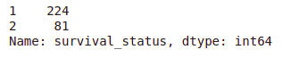
- The dataset is imbalanced as anticipated.
- Out of a complete of 305 sufferers, the variety of sufferers who survived over 5 years post-operation is sort of 3 occasions the variety of sufferers who died inside 5 years.
Checking for Lacking Values:
Let’s test for any lacking values within the dataset.
print("Lacking values in every column:n", df.isnull().sum())Output:

There are not any lacking values within the dataset.
Knowledge Info:
Let’s get a abstract of the dataset to know the info sorts and additional confirm the absence of lacking values.
df.information()Output:
- All of the columns are of integer sort.
- No lacking values within the dataset.
All columns are of integer sort.
By understanding the fundamental construction, distribution, and completeness of the info, we will proceed with extra detailed exploratory information evaluation (EDA) and uncover deeper insights.
Knowledge Preparation
Earlier than continuing with statistical evaluation and visualization, we have to modify the unique class labels. The present labels are 1 (survived 5 years or extra) and 2 (died inside 5 years), which aren’t very descriptive. We’ll map these to extra intuitive categorical variables: ‘sure’ for survival and ‘no’ for non-survival.
# Map survival standing values to categorical variables 'sure' and 'no'
df['survival_status'] = df['survival_status'].map({1: 'sure', 2: 'no'})

# Show the up to date DataFrame to confirm adjustments
print(df.head())
Basic Statistical Evaluation
We are going to now carry out a normal statistical evaluation to know the general distribution and central tendencies of the info.
# Show abstract statistics of the DataFrame
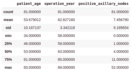
df .describe ()Output:
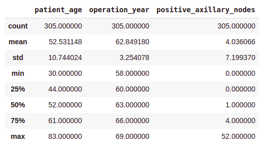
- On common, sufferers obtained operated at age of 63.
- A mean variety of constructive axillary nodes detected = 4.
- As indicated by the fiftieth percentile, the median of constructive axillary nodes is 1.
- As indicated by the seventy fifth percentile, 75% of the sufferers have lower than 4 nodes detected.
For those who see, there’s a important distinction between the imply and the median values. It’s because there are some outliers in our information and the imply is influenced by the presence of outliers.
Class-wise Statistical Evaluation
To achieve deeper insights, we’ll carry out a statistical evaluation for every class (survived vs. not survived) individually.
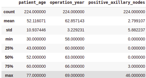
Survived (Sure) Evaluation:
survival_yes = df[df['survival_status'] == 'sure']
print(survival_yes.describe())
Output:
Not Survived (No) Evaluation:
survival_no = df[df['survival_status'] == 'no']
print(survival_no.describe())
Output:
From the above class-wise evaluation, it may be noticed that —
- The common age at which the affected person is operated on is sort of the identical in each instances.
- Sufferers who died inside 5 years on common had about 4 to five constructive axillary nodes greater than the sufferers who lived over 5 years post-operation.
Be aware that, all these observations are solely based mostly on the info at hand.
3. Uni-variate Knowledge Evaluation
“An image is price ten thousand phrases”
– Frank R. Bernard
Uni-variate evaluation entails learning one variable at a time. The sort of evaluation helps in understanding the distribution and traits of every variable individually. Beneath are alternative ways to carry out uni-variate evaluation together with their outputs and interpretations.
Distribution Plots
Distribution plots, often known as chance density perform (PDF) plots, present how values in a dataset are unfold out. They assist us see the form of the info distribution and determine patterns.
Affected person’s Age
sns.FacetGrid(information, hue="Survival_Status", peak=5).map(sns.histplot, "Age", kde=True).add_legend()
plt.title('Distribution of Age')
plt.xlabel('Age')
plt.ylabel('Frequency')
plt.present()
Output:
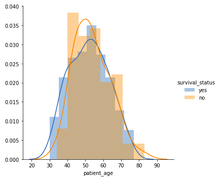
- Amongst all age teams, sufferers aged 40-60 years are the very best.
- There’s a excessive overlap between the category labels, implying that survival standing post-operation can’t be discerned from age alone.
Operation 12 months
sns.FacetGrid(information, hue="Survival_Status", peak=5).map(sns.histplot, "12 months", kde=True).add_legend()
plt.title('Distribution of Operation 12 months')
plt.xlabel('Operation 12 months')
plt.ylabel('Frequency')
plt.present()
Output:
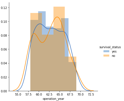
- Much like the age plot, there’s a important overlap between the category labels, suggesting that operation yr alone isn’t a particular issue for survival standing.
Variety of Optimistic Axillary Nodes
sns.FacetGrid(information, hue="Survival_Status", peak=5).map(sns.histplot, "Nodes", kde=True).add_legend()
plt.title('Distribution of Optimistic Axillary Nodes')
plt.xlabel('Variety of Optimistic Axillary Nodes')
plt.ylabel('Frequency')
plt.present()
Output:
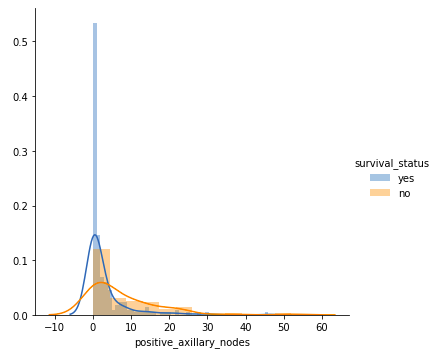
- Sufferers with 4 or fewer axillary nodes largely survived 5 years or longer.
- Sufferers with greater than 4 axillary nodes have a decrease probability of survival in comparison with these with 4 or fewer nodes.
However our observations have to be backed by some quantitative measure. That’s the place the Cumulative Distribution perform(CDF) plots come into the image.
Cumulative Distribution Perform (CDF)
CDF plots present the chance {that a} variable will take a price lower than or equal to a selected worth. They supply a cumulative measure of the distribution.
counts, bin_edges = np.histogram(information[data['Survival_Status'] == 1]['Nodes'], density=True)
pdf = counts / sum(counts)
cdf = np.cumsum(pdf)
plt.plot(bin_edges[1:], cdf, label="CDF Survival standing = Sure")

counts, bin_edges = np.histogram(information[data['Survival_Status'] == 2]['Nodes'], density=True)
pdf = counts / sum(counts)
cdf = np.cumsum(pdf)
plt.plot(bin_edges[1:], cdf, label="CDF Survival standing = No")

plt.legend()
plt.xlabel("Optimistic Axillary Nodes")
plt.ylabel("CDF")
plt.title('Cumulative Distribution Perform for Optimistic Axillary Nodes')
plt.grid()
plt.present()
Output:
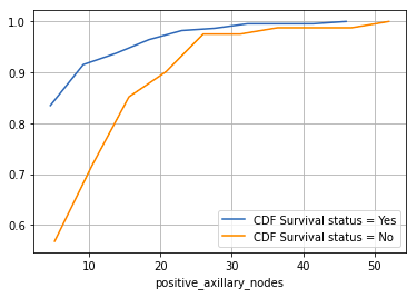
- Sufferers with 4 or fewer constructive axillary nodes have about an 85% likelihood of surviving 5 years or longer post-operation.
- The probability decreases for sufferers with greater than 4 axillary nodes.
Field Plots
Field plots, often known as box-and-whisker plots, summarize information utilizing 5 key metrics: minimal, decrease quartile (twenty fifth percentile), median (fiftieth percentile), higher quartile (seventy fifth percentile), and most. Additionally they spotlight outliers.
plt.determine(figsize=(15, 4))
plt.subplot(1, 3, 1)
sns.boxplot(x='Survival_Status', y='Age', information=information)
plt.title('Field Plot of Age')
plt.subplot(1, 3, 2)
sns.boxplot(x='Survival_Status', y='12 months', information=information)
plt.title('Field Plot of Operation 12 months')
plt.subplot(1, 3, 3)
sns.boxplot(x='Survival_Status', y='Nodes', information=information)
plt.title('Field Plot of Optimistic Axillary Nodes')
plt.present()
Output:
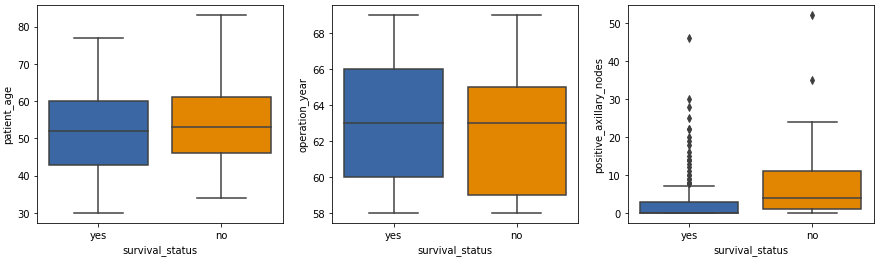
- The affected person age and operation yr plots present related statistics.
- The remoted factors within the constructive axillary nodes field plot are outliers, which is anticipated in medical datasets.
Violin Plots
Violin plots mix the options of field plots and density plots. They supply a visible abstract of the info and present the distribution’s form, density, and variability.
plt.determine(figsize=(15, 4))
plt.subplot(1, 3, 1)
sns.violinplot(x='Survival_Status', y='Age', information=information)
plt.title('Violin Plot of Age')
plt.subplot(1, 3, 2)
sns.violinplot(x='Survival_Status', y='12 months', information=information)
plt.title('Violin Plot of Operation 12 months')
plt.subplot(1, 3, 3)
sns.violinplot(x='Survival_Status', y='Nodes', information=information)
plt.title('Violin Plot of Optimistic Axillary Nodes')
plt.present()
Output:
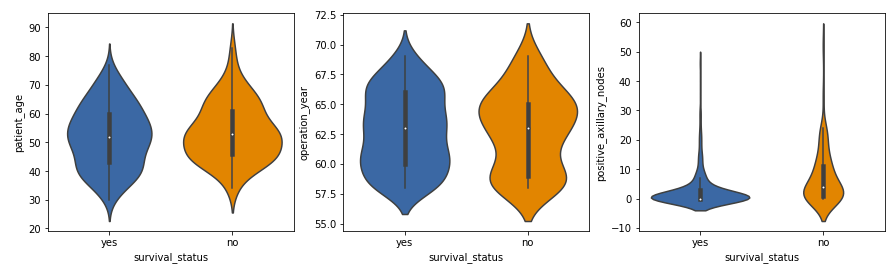
- The distribution of constructive axillary nodes is very skewed for the ‘sure’ class label and reasonably skewed for the ‘no’ label.
- The vast majority of sufferers, no matter survival standing, have a decrease variety of constructive axillary nodes, with these having 4 or fewer nodes extra more likely to survive 5 years post-operation.
These observations align with our earlier analyses and supply a deeper understanding of the info.
Bar Charts
Bar charts show the frequency or depend of classes inside a single variable, making them helpful for evaluating totally different teams.
Survival Standing Depend
sns.countplot(x='Survival_Status', information=df)
plt.title('Depend of Survival Standing')
plt.xlabel('Survival Standing')
plt.ylabel('Depend')
plt.present()
Output:

- This bar chart exhibits the variety of sufferers who survived 5 years or longer versus those that didn’t. It helps visualize the category imbalance within the dataset.
Histograms
Histograms present the distribution of numerical information by grouping information factors into bins. They assist perceive the frequency distribution of a variable.
Age Distribution
df['Age'].plot(type='hist', bins=20, edgecolor="black")
plt.title('Histogram of Age')
plt.xlabel('Age')
plt.ylabel('Frequency')
plt.present()
Output:

- The histogram shows how the ages of sufferers are distributed. Most sufferers are between 40 and 60 years outdated.
These observations align with our earlier analyses and supply a deeper understanding of the info.
4. Bi-variate Knowledge Evaluation
Bi-variate information evaluation entails learning the connection between two variables at a time. This helps in understanding how one variable impacts one other and may reveal underlying patterns or correlations. Listed below are some widespread strategies for bi-variate evaluation.
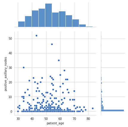
Pair Plot
A pair plot visualizes the pairwise relationships between variables in a dataset. It shows each the distributions of particular person variables and their relationships.
sns.set_style('whitegrid')
sns.pairplot(information, hue="Survival_Status")
plt.present()
Output:
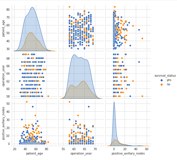
- The pair plot exhibits scatter plots of every pair of variables and histograms of every variable alongside the diagonal.
- The scatter plots on the higher and decrease halves of the matrix are mirror photos, so analyzing one half is adequate.
- The histograms on the diagonal present the univariate distribution of every function.
- There’s a excessive overlap between any two options, indicating no clear distinction between the survival standing class labels based mostly on function pairs.
Whereas the pair plot offers an summary of the relationships between all pairs of variables, typically it’s helpful to concentrate on the connection between simply two particular variables in additional element. That is the place the joint plot is available in.
Joint Plot
A joint plot offers an in depth view of the connection between two variables together with their particular person distributions.
sns.jointplot(x='Age', y='Nodes', information=information, type='scatter')
plt.present()
Output:
- The scatter plot within the heart exhibits no correlation between the affected person’s age and the variety of constructive axillary nodes detected.
- The histogram on the highest edge exhibits that sufferers usually tend to get operated on between the ages of 40 and 60 years.
- The histogram on the fitting edge signifies that almost all of sufferers had fewer than 4 constructive axillary nodes.
Whereas joint plots and pair plots assist visualize the relationships between pairs of variables, a heatmap can present a broader view of the correlations amongst all of the variables within the dataset concurrently.
Heatmap
A heatmap visualizes the correlation between totally different variables. It makes use of shade coding to characterize the power of the correlations, which might help determine relationships between variables.
sns.heatmap(information.corr(), cmap='YlGnBu', annot=True)
plt.present()
Output:

- The heatmap shows Pearson’s R values, indicating the correlation between pairs of variables.
- Correlation values near 0 counsel no linear relationship between the variables.
- On this dataset, there are not any robust correlations between any pairs of variables, as most values are close to 0.
These bi-variate evaluation methods present useful insights into the relationships between totally different options within the dataset, serving to to know how they work together and affect one another. Understanding these relationships is essential for constructing extra correct fashions and making knowledgeable selections in information evaluation and machine studying duties.
5. Multivariate Evaluation
Multivariate evaluation entails inspecting greater than two variables concurrently to know their relationships and mixed results. The sort of evaluation is crucial for uncovering complicated interactions in information. Let’s discover a number of multivariate evaluation methods.
Contour Plot
A contour plot is a graphical method that represents a three-dimensional floor by plotting fixed z slices, referred to as contours, in a 2-dimensional format. This enables us to visualise complicated relationships between three variables in an simply interpretable 2-D chart.
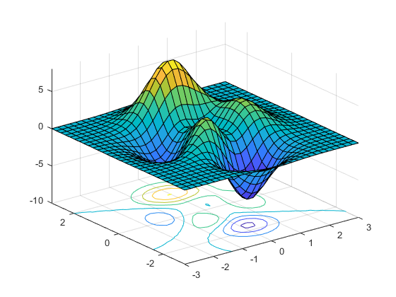
For instance, let’s look at the connection between affected person’s age and operation yr, and the way these relate to the variety of sufferers.
sns.jointplot(x='Age', y='12 months', information=information, type='kde', fill=True)
plt.present()
Output:

- From the above contour plot, it may be noticed that the years 1959–1964 witnessed extra sufferers within the age group of 45–55 years.
- The contour traces characterize the density of knowledge factors. Nearer contour traces point out a better density of knowledge factors.
- The areas with the darkest shading characterize the very best density of sufferers, exhibiting the commonest combos of age and operation yr.
By using contour plots, we will successfully consolidate data from three dimensions right into a two-dimensional format, making it simpler to determine patterns and relationships within the information. This strategy enhances our capability to carry out complete multivariate evaluation and extract useful insights from complicated datasets.
3D Scatter Plot
A 3D scatter plot is an extension of the standard scatter plot into three dimensions, which permits us to visualise the connection amongst three variables.
from mpl_toolkits.mplot3d import Axes3D

fig = plt.determine()
ax = fig.add_subplot(111, projection='3d')

ax.scatter(df['Age'], df['Year'], df['Nodes'])
ax.set_xlabel('Age')
ax.set_ylabel('12 months')
ax.set_zlabel('Nodes')

plt.present()
Output

- Most sufferers are aged between 40 to 70 years, with their surgical procedures predominantly occurring between the years 1958 to 1966.
- The vast majority of sufferers have fewer than 10 constructive axillary lymph nodes, indicating that low node counts are widespread on this dataset.
- Just a few sufferers have a considerably increased variety of constructive nodes (as much as round 50), suggesting instances of extra superior most cancers.
- There is no such thing as a robust correlation between the affected person’s age or the yr of surgical procedure and the variety of constructive nodes detected. Optimistic nodes are unfold throughout varied ages and years with out a clear development.
Conclusion
On this article, we discovered some widespread steps concerned in exploratory information evaluation. We additionally noticed a number of varieties of charts & plots and what data is conveyed by every of those. That is simply not it, I encourage you to play with the info and provide you with totally different sorts of visualizations and observe what insights you may extract from it.
Key Takeaways:
- EDA is essential for understanding information, figuring out points, and extracting insights earlier than modeling
- Varied methods like visualizations, statistical summaries, and information cleansing are utilized in EDA
- Python libraries like pandas, NumPy, Matplotlib, and Seaborn are generally used for EDA
The media proven on this article will not be owned by Analytics Vidhya and are used on the Writer’s discretion.
Continuously Requested Questions
A. Exploratory information evaluation (EDA) is the preliminary investigation of knowledge to summarize its most important traits, usually utilizing visible strategies.
A. Knowledge exploration evaluation entails inspecting datasets to uncover patterns, anomalies, and relationships, offering insights for additional evaluation.
A. EDA is used to know information distributions, determine outliers, uncover patterns, and inform the selection of statistical instruments and methods.
A. Steps of EDA embody: information cleansing, summarizing statistics, visualizing information, figuring out patterns, and producing hypotheses for additional evaluation.